
I was writing C++ code for convolutions and expected it to work as fast as Pytorch. The result - my Conv implementation was 100x slower than PyTorch. I even compared no of FLOPs of my code with Pytorch. But, no difference there. After days of optimizing C++ code, I realised my code was slow because in frameworks convolutions are not implemented the way we visualise them. Even though FLOPs are same, fetching data from memory is way slower and more energy-consuming in traditional convolution. Actual convolutions are implemented after im2col kernel transformations through GEMM operations. If you have never heard of them before, you are at the right place. We'll be demystifying them here.
But before getting into it, look at this table.
The interesting thing in this image is that energy consumption of ALU op (part of CPU which do all computation) is 1000x less than data movement from DRAM. Processing time also has a similar trend. Usually, for calculating processing time, we calculate no of computations but not realize that in data-intensive operations, communication (data movement) plays a major role. It’s not enough to just compute the data fast if we can’t get the data fast. Let's start with basics -
Data layout - Data layout defines how multidimensional matrices are stored in memory. For a 2-D array, it can either be row-major or column-major order. In row-major order, the consecutive elements of a row reside next to each other, whereas the same holds true for consecutive elements of a column in column-major order. Data layout is important for performance when traversing an array because modern CPUs process sequential data more efficiently than nonsequential data. This is primarily due to CPU caching.

Source: Wikipedia
CPU caching - The RAM is large but slow storage. CPU caches are orders of magnitude faster, but much smaller. When trying to read or write some data, the processor checks whether the data is already in the cache. If so, the processor will read from or write to the cache instead of the much slower main memory. Every time we fetch data from the main memory, the CPU automatically loads it and its neighbouring memory into the cache, hoping to utilize locality of reference.
Locality of Reference -
Spatial locality - It is highly likely that any consecutive storage in memory might be referenced sooner. That's why if a[i] is needed, CPU also prefetches a[i+1], a[i+2], ... in cache. Temporal locality - It is highly likely that if some variable is accessed by the program, they will be referenced again. That's why recently used variables are stored in the cache after computation.
Okay. So now, we have to optimize our code in such a way that either the data recently used will be used again or the data sequentially near that data will be used. Let's first look at traditional convolution operation -
for filter in 0..num_filters
    for channel in 0..input_channels
        for out_h in 0..output_height
            for out_w in 0..output_width
                for k_h in 0..kernel_height
                    for k_w in 0..kernel_width
                        output[filter, out_h, out_w] +=
                            kernel[filter, channel, k_h, k_w] *
                            input[channel, out_h + k_h, out_w + k_w]
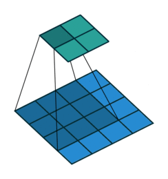
For input image of shape (4,4, 2) and filter of shape (3,3, 2).

Data access pattern when (3,3,2) filter is placed on (4,4,2) image.
Above diagram shows how memory is accessed for the first window of the convolution operation. When we are at (0,0), CPU loads data not only for (0,0) but also for the next elements of the row in the cache. So, it won't need to load data from memory at (0,1) and (0,2) because they are already in cache. But, when we are at (0,2), next element i.e (1,0) is not in cache - we get a cache miss and CPU stalls while the data is fetched. Similarly, it keeps stalling at (1,2), (2,2), etc. So, what im2col does is simply arrange elements of one convolution window in one row. Then, they can be accessed sequentially from the cache without jumping. So, all 18 elements required for convolution are rearranged as in figure below.

In our example, there will be four Conv windows, after converting all to im2col and stacking over, we get following 2-D array.

input activations after im2col
As you can see, now we have 18x4= 72 elements instead of 32 elements (in the original image). That's the downside of im2col but with performance difference, it's all worth it. We also need to rearrange filters (Actually, they are already stored like this). The full process can be visualized from the following image by Leonardo.
After rearranging image, we also need to rearrange filters (In practice, they are already stored like this). Suppose we had 5 filters of (3,3,2), then each filter will be arranged into a single column. Then 5 of them are stacked to get (18, 5) matrix.

filters (18,5)
Now, we have converted this into a simple 2-D matrix multiplication problem. And this is a very common problem in scientific computing. There exist BLAS libraries like OpenBLAS, Eigen, Intel MKL for computing GEMM (General Element Matrix Multiplications). These libraries have been optimized for many decades for matrix multiplication and are now used in all frameworks like Tf, Pytorch etc.

Matrix multiplication of input and filter gives the resultant matrix of shape (4,5). Now, this can be rearranged into (2,2,5) matrix which is our expected size. Finally, after using im2col, I could get speeds only 2-3x slower than Pytorch. But it's not the end of the story. There are also some other algorithms like -
Winograd Fast convolution - Reduces no. of multiplications by 2.5x on 3x3 filter. But works well on small filters only. Fast Fourier Transformation - Improves speed only on very large filters and batch size. Strassen's algorithm - It reduces the number of multiplications from O( N^3) to O( N^2.807). But increase storage requirements and reduced numerical stability.